Polynomials |
Why did we introduce such alleged complicated functionality into SERVOsoft? The answer is with Polynomials, we can solve almost any motion task, and it is one basis for the Optimizer.
So let us start with some mathematics and we’ll soon realize that in the end we can concentrate on our motion application and our well known variables time, distance, speed, acceleration, jerk etc., with all necessary calculations done automatically by SERVOsoft.
A polynomial (of n-th order) is a mathematical function of the form
![]()
Often the term 'Polynomial' is shortened to 'Poly', and the names are shortened to 'Poly 1-3', 'Poly 1-5' and 'Poly 1-7'. Polynomials 345 and 4567 are subsets of the full polynomials with the first terms set to zero. Poly 345 and 4567, which have been used in SERVOsoft since the beginning, are 'ramp' profiles where the start and end acceleration values are always zero.
For Poly 1-5 and Poly 1-7, which have the first terms, a lot more flexibility is possible. For example, Poly 1-5 allows the user to specify the start and end velocity, and the start and end acceleration. And for Poly 1-7, users can also specify the start and end jerk values.
When n=5 or 7, they are often called a 'Polynomial of 5th Degree' or 'Polynomial of 7th Degree' respectively. Because SERVOsoft also uses the 'ramp' polynomials 345 and 4567, the naming convention clearly states the terms. Ie. Either 'Poly 345', which is the 'ramp' profile, or 'Poly 12345', which has all terms.
But let’s start simple, the 1st order polynomial commonly is known as Straight Line
![]()
So if we set x as time and p(x) as distance, this will be for example a segment with
| with | and |
But as you can see the segment is defined in SERVOsoft as
Polynomial 123, which means as 3rd order
polynomial![]() with the four variables
Time, Distance, Start
Velocity and End Velocity.
with the four variables
Time, Distance, Start
Velocity and End Velocity.
So how does it come that this defines our straight line? Well
first when we deal with a 3rd order polynomial we need to know what
the values of the four unknown coefficients ![]() are.
are.
Remembering our Linear Algebra lessons we need four equations to solve for four unknowns (and we can leave out the units):
| (eqn1, i.e. we want to start at |
||
| (eqn2, i.e. the distance to travel in |
||
| (eqn3, i.e. the start velocity is |
||
| (eqn4, i.e. the end velocity is |
Now let’s do it one time in detail (note in each new line we take
the results of the previous lines into account):
| (eqn1) | |||||||
| (eqn3) | |||||||
| (eqn2) | (eqn2a) | ||||||
| (eqn4) | (eqn4a) |
3 * (eqn2a) –
(eqn4a) -> ![]() and with
(eqn2a) ->
and with
(eqn2a) -> ![]()
And we are done with ![]() , which is our unique
straight line.
, which is our unique
straight line.
This leads us to our first theorem which will make our life much easier when dealing with polynomials. Because Linear Algebra says: To solve for a number of unknowns you will need the same number of equations, i.e. for a 3rd order polynomial with four unknown coefficients we will need four equations or generally spoken constraints.
A n-th order polynomial is uniquely described by n+1 constraints
This theorem tells us that we don’t need anything to know about coefficients, we only need to know about our applications constraints in order to define polynomial segments, the needed mathematical calculations are all done by SERVOsoft under the hood.
So let us keep this in mind:
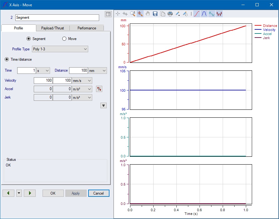
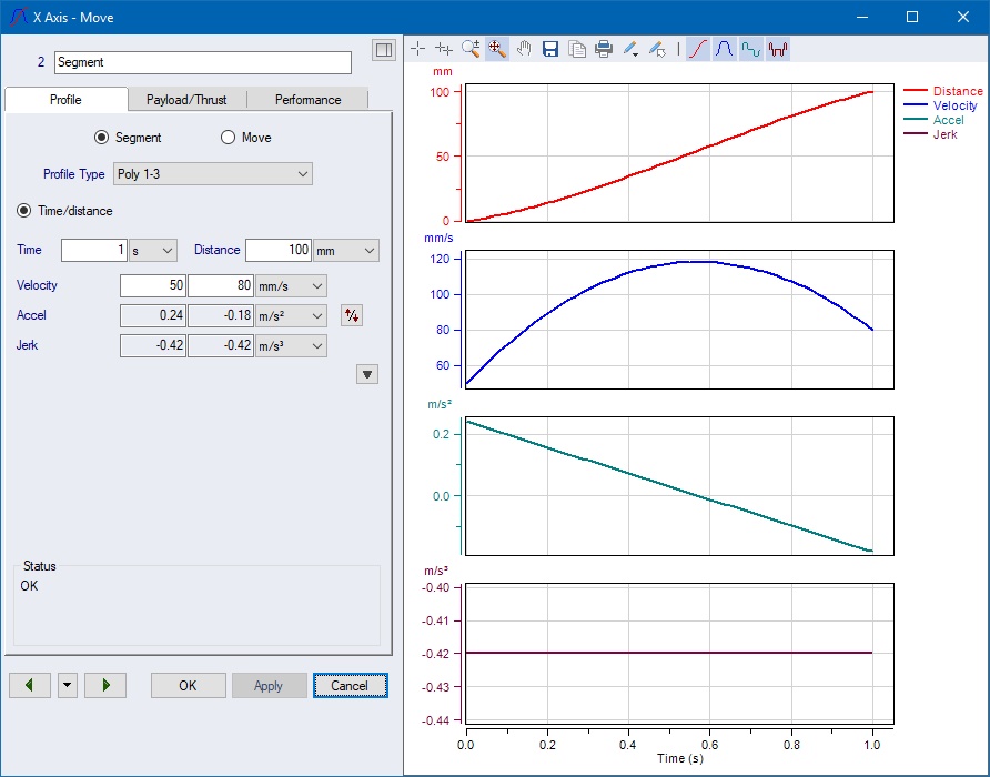
As an example a Polynomial 123 with the set
four values Time = 1 s, Distance = 100 mm, Start
Velocity = ![]() and
End Velocity =
and
End Velocity = ![]() will
uniquely look like this:
will
uniquely look like this:
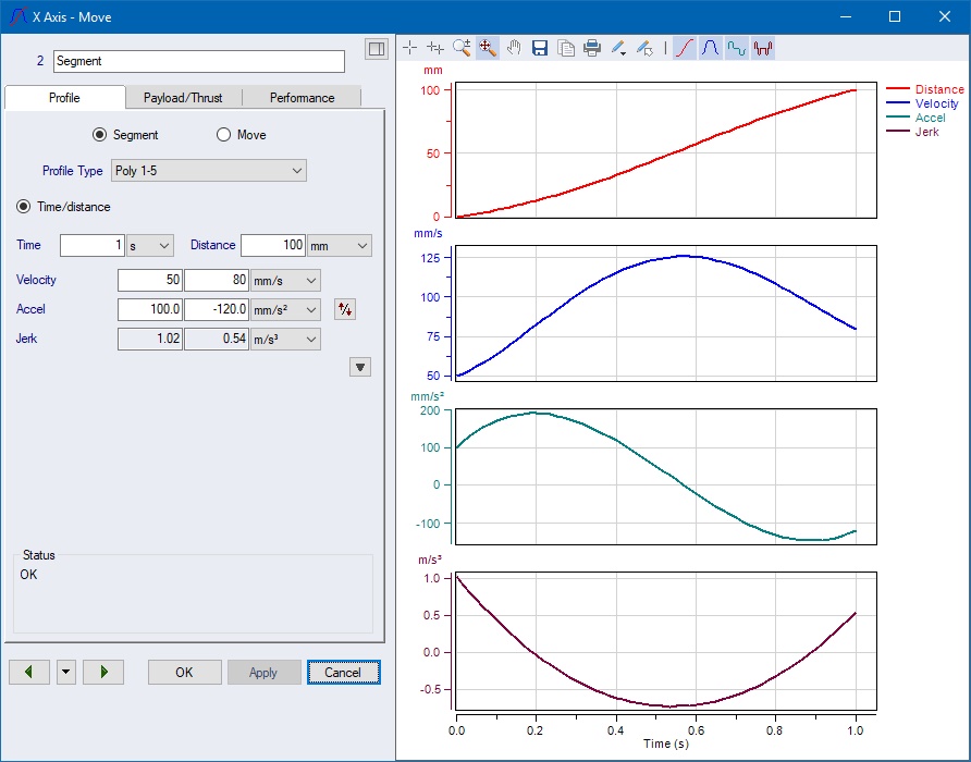
A Polynomial 12345 with the set six values Time
= 1 s, Distance = 100 mm, Start Velocity = ![]() , End
Velocity =
, End
Velocity = ![]() , Start
Acceleration =
, Start
Acceleration = ![]() and
End Acceleration =
and
End Acceleration = ![]() will
uniquely look like this:
will
uniquely look like this:
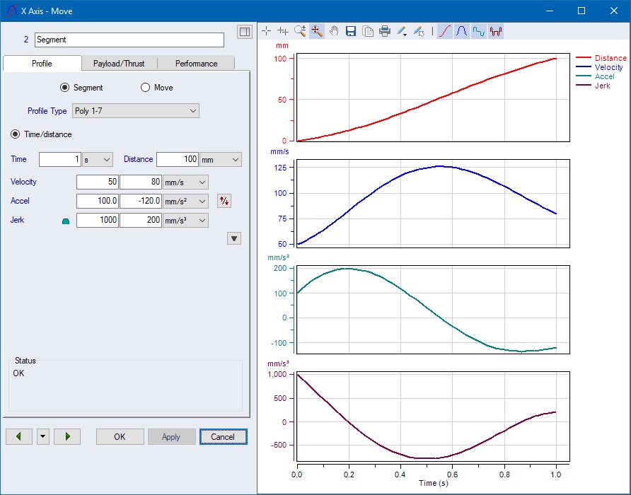
A Polynomial 1234567 with the set eight values
Time = 1 s, Distance = 100 mm, Start Velocity = ![]() , End
Velocity =
, End
Velocity = ![]() , Start
Acceleration =
, Start
Acceleration = ![]() ,
End Acceleration =
,
End Acceleration = ![]() , Start
Jerk =
, Start
Jerk = ![]() and
End Jerk =
and
End Jerk = ![]() will
uniquely look like this:
will
uniquely look like this: